Hemispherical Signed Distance Field Ambient Occlusion
Introduction
Raymarching by distance field was introduced by John C. Hart in this paper and became more popular in 2008 with this presentation by Inigo Quilez.
Alex Evans got an Ambient Occlusion technique based on signed distance field (SDF) surface in 2006 (paper).
The classical method
The idea is to sample the SDF along the normal vector and get the difference between the SDF and the real distance to our point. The more the sampled SDF is small, the more the object are occluded.
Considering to a point p with the normal n, a random function hash(i) in [0..1] and a function map(x,y,z) which is our distance field, we can write this :
float ambientOcclusion( in vec3 p, in vec3 n, in float maxDist, in float falloff )
{
    float ao = 0.0;
    const int nbIte = 6;
    for( int i=0; i<nbIte; i++ )
    {
        float l = hash(float(i))*maxDist;
        vec3 rd = n*l;

        ao += (l - max(map( p + rd ),0.)) / maxDist * falloff;
    }

    return clamp( 1.-ao/float(nbIte), 0., 1.);
}
So, we marching along the normal at a random length and getting the difference between our two distances and divide this by a falloff factor based on the real distance to our point.
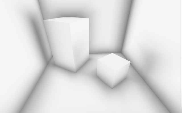
We obtain a good noise free results with few step (like 6) :
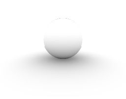
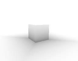
The AO on the sphere image seems to be quite perfect but on the cube it doesn't. We can see more AO if we follow the edges of the cube on the floor. This solution is only suitable for rounded surfaces.
Improved AO by hemispherical sampling
Back to the root, in classic raytracing we get AO by tracing rays to the point with an hemispherical direction along the normal.
You can obtain perfect result with this technique but you must send many rays (like 5000) to get it noise free.
So the idea is just to combine the both : taking samples of the SDF in an hemispherical direction along the normal. We just have to add one function to get a random hemispherical direction and modify the classical method a little bit:
vec3 randomSphereDir(vec2 rnd)
{
    float s = rnd.x*PI*2.;
    float t = rnd.y*2.-1.;
    return vec3(sin(s), cos(s), t) / sqrt(1.0 + t * t);
}
vec3 randomHemisphereDir(vec3 dir, float i)
{
    vec3 v = randomSphereDir( vec2(hash(i+1.), hash(i+2.)) );
    return v * sign(dot(v, dir));
}
float ambientOcclusion( in vec3 p, in vec3 n, in float maxDist, in float falloff )
{
    const int nbIte = 32;
    const float nbIteInv = 1./float(nbIte);
    const float rad = 1.-1.*nbIteInv; //Hemispherical factor (self occlusion correction)

    float ao = 0.0;

    for( int i=0; i<nbIte; i++ )
    {
        float l = hash(float(i))*maxDist;
        vec3 rd = normalize(n+randomHemisphereDir(n, l )*rad)*l; // mix direction with the normal for self occlusion problems!

        ao += (l - max(map( p + rd ),0.)) / maxDist * falloff;
    }

    return clamp( 1.-ao*nbIteInv, 0., 1.);
}
Of course we need more iteration than the classical method but only 16 samples already provide good results!
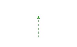
As you see, I mixed the hemispherical direction and the normal by a "rad" factor based on the number of iterations. This is because of the self occlusion problem :
If we sample this point in blue, we will get the small distance in red which is very small compared to the distance to our original point p. The less iterations you have, the more this self occlusion will be a problem. So when we have small number of iterations, we just tend to the classical method and march more along the normal.
You can compare the classical method and the hemispherical method in real time (go to Shadertoy to view the source code) :